you’ll take a look how the gradient for logistic cost is calculated in code. This will be useful to look at because you will implement this in the practice lab at the end of the week.
After you run gradient descent in the lab, there will be a nice set of animated plots that show gradient descent in action. You’ll see the sigmoid function, the contour plot of the cost, the 3D surface plot of the cost, and the learning curve all evolve as gradient descent runs
This is my learning experience of data science through DeepLearning.AI. These repository contributions are part of my learning journey through my graduate program masters of applied data sciences (MADS) at University Of Michigan, DeepLearning.AI, Coursera & DataCamp. You can find my similar articles & more stories at my medium & LinkedIn profile. I am available at kaggle & github blogs & github repos. Thank you for your motivation, support & valuable feedback.
These include projects, coursework & notebook which I learned through my data science journey. They are created for reproducible & future reference purpose only. All source code, slides or screenshot are intellectual property of respective content authors. If you find these contents beneficial, kindly consider learning subscription from DeepLearning.AI Subscription, Coursera, DataCamp
Optional Lab: Gradient Descent for Logistic Regression
Goals
In this lab, you will: - update gradient descent for logistic regression. - explore gradient descent on a familiar data set
As before, we’ll use a helper function to plot this data. The data points with label \(y=1\) are shown as red crosses, while the data points with label \(y=0\) are shown as blue circles.
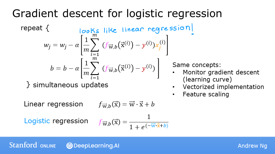
Where each iteration performs simultaneous updates on \(w_j\) for all \(j\), where \[\begin{align*}
\frac{\partial J(\mathbf{w},b)}{\partial w_j} &= \frac{1}{m} \sum\limits_{i = 0}^{m-1} (f_{\mathbf{w},b}(\mathbf{x}^{(i)}) - y^{(i)})x_{j}^{(i)} \tag{2} \\
\frac{\partial J(\mathbf{w},b)}{\partial b} &= \frac{1}{m} \sum\limits_{i = 0}^{m-1} (f_{\mathbf{w},b}(\mathbf{x}^{(i)}) - y^{(i)}) \tag{3}
\end{align*}\]
m is the number of training examples in the data set
\(f_{\mathbf{w},b}(x^{(i)})\) is the model’s prediction, while \(y^{(i)}\) is the target
For a logistic regression model \(z = \mathbf{w} \cdot \mathbf{x} + b\)\(f_{\mathbf{w},b}(x) = g(z)\) where \(g(z)\) is the sigmoid function: \(g(z) = \frac{1}{1+e^{-z}}\)
Gradient Descent Implementation
The gradient descent algorithm implementation has two components: - The loop implementing equation (1) above. This is gradient_descent below and is generally provided to you in optional and practice labs. - The calculation of the current gradient, equations (2,3) above. This is compute_gradient_logistic below. You will be asked to implement this week’s practice lab.
Calculating the Gradient, Code Description
Implements equation (2),(3) above for all \(w_j\) and \(b\). There are many ways to implement this. Outlined below is this: - initialize variables to accumulate dj_dw and dj_db - for each example - calculate the error for that example \(g(\mathbf{w} \cdot \mathbf{x}^{(i)} + b) - \mathbf{y}^{(i)}\) - for each input value \(x_{j}^{(i)}\) in this example, - multiply the error by the input \(x_{j}^{(i)}\), and add to the corresponding element of dj_dw. (equation 2 above) - add the error to dj_db (equation 3 above)
divide dj_db and dj_dw by total number of examples (m)
note that \(\mathbf{x}^{(i)}\) in numpy X[i,:] or X[i] and \(x_{j}^{(i)}\) is X[i,j]
Code
def compute_gradient_logistic(X, y, w, b):""" Computes the gradient for linear regression Args: X (ndarray (m,n): Data, m examples with n features y (ndarray (m,)): target values w (ndarray (n,)): model parameters b (scalar) : model parameter Returns dj_dw (ndarray (n,)): The gradient of the cost w.r.t. the parameters w. dj_db (scalar) : The gradient of the cost w.r.t. the parameter b. """ m,n = X.shape dj_dw = np.zeros((n,)) #(n,) dj_db =0.for i inrange(m): f_wb_i = sigmoid(np.dot(X[i],w) + b) #(n,)(n,)=scalar err_i = f_wb_i - y[i] #scalarfor j inrange(n): dj_dw[j] = dj_dw[j] + err_i * X[i,j] #scalar dj_db = dj_db + err_i dj_dw = dj_dw/m #(n,) dj_db = dj_db/m #scalarreturn dj_db, dj_dw
Check the implementation of the gradient function using the cell below.
The code implementing equation (1) above is implemented below. Take a moment to locate and compare the functions in the routine to the equations above.
Code
def gradient_descent(X, y, w_in, b_in, alpha, num_iters):""" Performs batch gradient descent Args: X (ndarray (m,n) : Data, m examples with n features y (ndarray (m,)) : target values w_in (ndarray (n,)): Initial values of model parameters b_in (scalar) : Initial values of model parameter alpha (float) : Learning rate num_iters (scalar) : number of iterations to run gradient descent Returns: w (ndarray (n,)) : Updated values of parameters b (scalar) : Updated value of parameter """# An array to store cost J and w's at each iteration primarily for graphing later J_history = [] w = copy.deepcopy(w_in) #avoid modifying global w within function b = b_infor i inrange(num_iters):# Calculate the gradient and update the parameters dj_db, dj_dw = compute_gradient_logistic(X, y, w, b)# Update Parameters using w, b, alpha and gradient w = w - alpha * dj_dw b = b - alpha * dj_db# Save cost J at each iterationif i<100000: # prevent resource exhaustion J_history.append( compute_cost_logistic(X, y, w, b) )# Print cost every at intervals 10 times or as many iterations if < 10if i% math.ceil(num_iters /10) ==0:print(f"Iteration {i:4d}: Cost {J_history[-1]} ")return w, b, J_history #return final w,b and J history for graphing
fig,ax = plt.subplots(1,1,figsize=(5,4))# plot the probabilityplt_prob(ax, w_out, b_out)# Plot the original dataax.set_ylabel(r'$x_1$')ax.set_xlabel(r'$x_0$')ax.axis([0, 4, 0, 3.5])plot_data(X_train,y_train,ax)# Plot the decision boundaryx0 =-b_out/w_out[0]x1 =-b_out/w_out[1]ax.plot([0,x0],[x1,0], c=dlc["dlblue"], lw=1)plt.show()
In the plot above: - the shading reflects the probability y=1 (result prior to decision boundary) - the decision boundary is the line at which the probability = 0.5
Another Data set
Let’s return to a one-variable data set. With just two parameters, \(w\), \(b\), it is possible to plot the cost function using a contour plot to get a better idea of what gradient descent is up to.
As before, we’ll use a helper function to plot this data. The data points with label \(y=1\) are shown as red crosses, while the data points with label \(y=0\) are shown as blue circles.
In the plot below, try: - changing \(w\) and \(b\) by clicking within the contour plot on the upper right. - changes may take a second or two - note the changing value of cost on the upper left plot. - note the cost is accumulated by a loss on each example (vertical dotted lines) - run gradient descent by clicking the orange button. - note the steadily decreasing cost (contour and cost plot are in log(cost) - clicking in the contour plot will reset the model for a new run - to reset the plot, rerun the cell